Gage R&R Acceptance Criteria: What Japanese Customers Expect

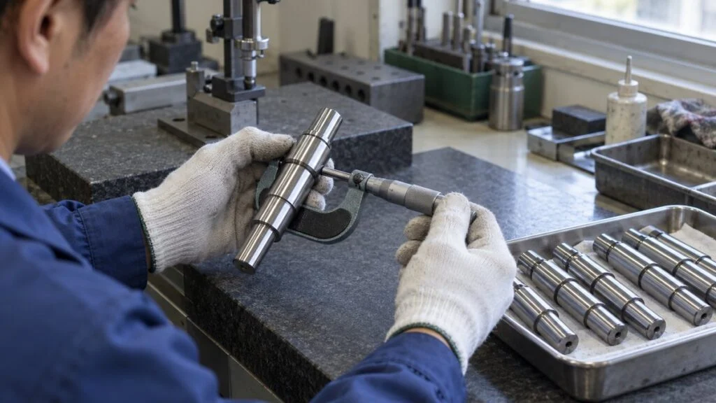
Your gauges are calibrated every year, and the certificates are on file. Then the Japanese customer's quality assurance team asks for gauge R&R results (written ゲージR&R in Japanese documents), or for your sokutei shisutemu kaiseki (測定システム解析, measurement systems analysis, MSA). Suppliers to Japanese automakers and Tier 1s, whether in Thailand, India, or the US, can expect this request at some point.

Calibration mainly checks one thing: how far the gauge reads from a reference standard (bias). Real measurements also scatter when the same person measures the same part again, and they shift when a different person takes over. Gage R&R puts a number on that scatter and compares it with the part-to-part variation or the tolerance.

This guide covers where Gage R&R sits inside MSA, the six steps of a study, a fully worked (fictional) example using the average and range method, how ANOVA results differ, and how to read the 10% and 30% acceptance criteria. It ends with the points Japanese customers tend to check, a pre-submission checklist, and questions to ask before you run the study.

Contents

1. What Gage R&R Measures Within MSA
2. How to Run a Gage R&R Study in 6 Steps
3. Average and Range Method: A Worked Example
4. Average and Range vs. ANOVA
5. Acceptance Criteria: Reading 10%, 30%, and ndc ≥ 5
6. What to Do When the Result Is Poor
7. Attribute MSA: Pass/Fail Inspection and Kappa
8. Before You Submit: Checklist and Questions for the Japanese Customer
9. Limits of This Guide
10. FAQ
11. Sources

What Gage R&R Measures Within MSA

MSA evaluates the whole measurement system statistically, not just the instrument. The system includes the person measuring, the method, the fixture, and the environment. In the automotive industry, the de facto standard is the MSA reference manual published by AIAG (Automotive Industry Action Group, the US automotive industry association). The current edition is the 4th, published in June 2010, and it is still the edition AIAG lists as of October 2026.

The manual splits measurement system error into two kinds: location error, where the average reading differs from the true value, and width (spread) error, where readings scatter around their average. Gage R&R evaluates the width error: how much the readings spread when you measure the same thing repeatedly.

Figure 1: The Five Properties MSA Evaluates

Three properties describe location error and two describe width error. Gage R&R combines the two width properties.

Bias

LocationDifference between the average reading and the reference value. Checked by calibration or by measuring a master part

Linearity

LocationWhether bias changes between the low and high ends of the measuring range

Stability

LocationWhether bias changes over time when the same master is measured at intervals. Tracked on a control chart

Repeatability (EV)

WidthVariation when one person measures the same part repeatedly with the same gauge. Also called equipment variation

Reproducibility (AV)

WidthDifference in average readings between appraisers. Also called appraiser variation

Gage R&R (GRR)

CombinedRepeatability and reproducibility combined: the width error of the measurement system

EV = equipment variation; AV = appraiser variation. Classification based on explanatory material that summarizes the AIAG MSA manual, 4th edition.

Repeatability and Reproducibility: A Note on Japanese Terms

Japanese reports use 繰返し性 (kurikaeshi-sei) for repeatability and 再現性 (saigen-sei) for reproducibility. The Japanese metrology vocabulary standard, JIS Z 8103, defines repeatability as precision under repeatability conditions: the same procedure, operator, measuring system, operating conditions, and location, with repeated measurements of the same object over a short period. Gage R&R reports this as EV.

The JIS definition of reproducibility is broader. Its reproducibility conditions can include different locations and different measuring systems. In Gage R&R, reproducibility (AV) mainly means the difference caused by changing the appraiser. If your procedure or report is going to a Japanese customer, it helps to state explicitly that "reproducibility = difference between appraisers" so nobody reads it in the wider JIS sense.

The study splits the total observed variation into variation from the parts themselves and variation from the measurement system, as shown below.

Figure 2: How Measurement Variation Breaks Down

In a good measurement system, part variation makes up most of the total variation and GRR is small.

Total variation (TV)All the variation seen in the readings. TV² = PV² + GRR²

Split into

Part variation (PV)Real dimensional differences between parts. The variation you want to see

Gage R&R (GRR)Variation from the measurement system. GRR² = EV² + AV²

GRR consists of

Repeatability (EV)Within-person variation from the gauge, fixture, and method

Reproducibility (AV)Differences in average readings between appraisers

Only variances (standard deviation squared) add. Standard deviations and percentages cannot simply be added together.

Calibration vs. Gage R&R

Calibration compares a gauge with a traceable standard and checks the error in its reading. It looks at the instrument alone, mainly the bias in Figure 1. Even with calibration and traceability in place, play in the fixture or habits of the person measuring still add variation. For more on calibration and traceability records at Japanese plants, see JCSS Calibration: Certificates, Intervals, and Records.

Gage R&R uses real parts, measured by the people who normally measure them, using the normal procedure. Calibration asks "Is the gauge correct?" Gage R&R asks "Can this measurement method tell the parts apart?" You need both before you can use the readings for quality decisions.

Why Japanese Automotive Customers Ask for It: IATF 16949 7.1.5.1.1

IATF 16949, the automotive quality management standard, requires MSA in clause 7.1.5.1.1. Statistical studies must analyze the variation in the results of each type of inspection, measurement, and test equipment system listed in the control plan. The analysis methods and acceptance criteria must follow the MSA reference manuals. Other methods or criteria are allowed only with customer approval, and records of that approval must be kept.

So the scope comes from the control plan, and the customer's own rules matter as much as the AIAG numbers. Where MSA sits in a Japanese customer's launch process is covered in Japanese NPI Process: 8 Steps to Mass Production and Quality Assurance Process at Japanese Plants.

How to Run a Gage R&R Study in 6 Steps

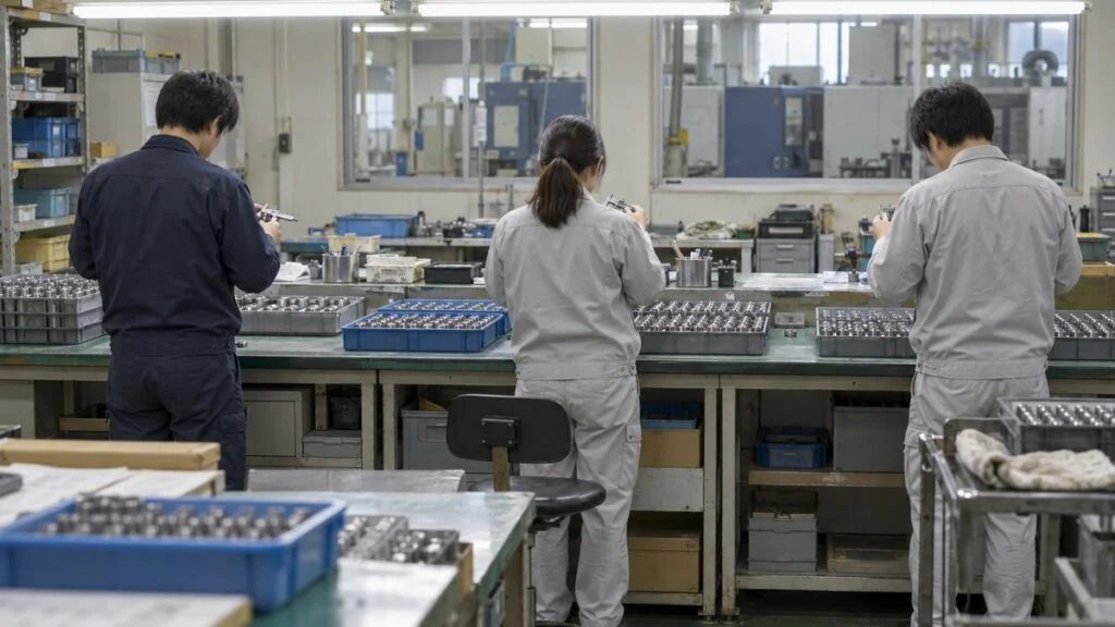
The quality of the data collection decides how much you can trust the result, more than the calculation does. Here is a typical plan with 10 parts, 3 appraisers, and 3 trials each, broken into six steps.

Figure 3: The Six Steps of a Gage R&R Study

The three preparation steps largely decide whether the result can be trusted.

Preparation

01Define the target and purposeWhich characteristic, which gauge. Process control or pass/fail inspection?

02Check resolution and calibrationIs the smallest increment 1/10 of the tolerance (or process variation) or finer? Is calibration current?

03Select partsAbout 10 parts covering the full process range. Number them so appraisers cannot see the numbers

Measurement and analysis

04Measure in random order3 appraisers, 3 trials each. Change the order every trial and hide earlier readings

05CalculateFind EV, AV, and GRR by the average and range (X̄-R) method or ANOVA

06Judge and actCompare %GRR and ndc with the criteria. If they fail, find out whether repeatability or reproducibility is the cause

10 parts, 2–3 appraisers, and 2–3 trials is a common guideline (Minitab technical paper). Follow the customer's specification if there is one.

Step 1: Define the Target and Purpose

Decide which quality characteristic you will study, and with which gauge, fixture, and procedure. Under IATF 16949, it is common to start with the measurements listed in the control plan. Also decide what the measurement is used for: tracking process variation on a control chart, or making pass/fail decisions before shipment. The answer changes which denominator you use for %GRR later.

Step 2: Check Resolution and Calibration

If the gauge's resolution (smallest readable increment) is too coarse, it returns the same reading every time and the variation cannot be evaluated properly. AIAG guidance includes the "10-to-1 rule": resolution should be one-tenth of the tolerance or finer. For a dimension with a 0.10 mm tolerance, you need a gauge that reads to 0.01 mm or better.

Confirm that the gauge's calibration is current. Gage R&R does not evaluate bias, so a good result from a gauge whose calibration is overdue does not prove the readings are correct.

Step 3: Select Parts

Choose parts that cover the whole range of variation the process actually produces. Minitab notes that sampling across the full process range gives a better estimate of part-to-part variation. If you collect similar parts from a single lot instead, part variation shrinks and %GRR comes out unfairly high.

Number the parts, but keep the numbers hidden from the appraisers. Appraisers who can see the number tend to remember their last reading and match it, so mark the underside of the part or have someone else hand the parts over. Ten parts do not estimate part variation very precisely. Minitab's technical paper gives two options: use more parts, or use a process standard deviation calculated from a large set of historical data.

Step 4: Measure in Random Order

Pick appraisers from the people who normally do this measurement. If you use only your best inspector, the study understates the variation in day-to-day measurement.

For trial 1, appraiser A measures all 10 parts once, then B and C do the same. Trials 2 and 3 repeat this with the part order shuffled. Randomizing the order every trial and keeping earlier results out of sight removes the effects of memory and measuring order. Agree in advance on exactly where on the part to measure, and make sure everyone uses the same location.

Steps 5 and 6: Calculate and Judge

Once the data is in, calculate with the average and range method or ANOVA. A spreadsheet can do it, but statistical software produces ANOVA results and graphs in one pass. To judge the result, compare %GRR and ndc (number of distinct categories) with the criteria. If they fail, check whether repeatability or reproducibility is larger and act on that. The next section walks through the calculation step by step.

Average and Range Method: A Worked Example

The data below is fictional. All numbers were made up for explanation and do not come from a real process. The setup: shaft outside diameter, specification 10.00 ±0.05 mm (tolerance width 0.10 mm), measured with a micrometer that reads to 0.001 mm. Appraisers A, B, and C each measure 10 parts three times.

Appraiser / trial	1	2	3	4	5	6	7	8	9	10
A, trial 1	9.972	9.986	10.020	9.995	10.029	9.962	10.008	9.994	10.014	10.000
A, trial 2	9.973	9.986	10.021	9.995	10.030	9.967	10.004	9.989	10.009	9.998
A, trial 3	9.966	9.984	10.017	9.999	10.030	9.964	10.000	9.988	10.015	10.002
A, range	0.007	0.002	0.004	0.004	0.001	0.005	0.008	0.006	0.006	0.004
B, trial 1	9.969	9.986	10.020	9.998	10.035	9.965	10.010	9.995	10.015	10.004
B, trial 2	9.974	9.987	10.019	10.000	10.036	9.962	10.013	9.992	10.015	10.010
B, trial 3	9.976	9.983	10.023	10.002	10.031	9.969	10.010	9.994	10.021	10.002
B, range	0.007	0.004	0.004	0.004	0.005	0.007	0.003	0.003	0.006	0.008
C, trial 1	9.969	9.980	10.017	9.990	10.024	9.960	10.007	9.989	10.007	9.996
C, trial 2	9.970	9.975	10.016	9.994	10.030	9.963	10.003	9.985	10.010	10.003
C, trial 3	9.967	9.980	10.018	9.994	10.025	9.958	10.004	9.985	10.014	10.000
C, range	0.003	0.005	0.002	0.004	0.006	0.005	0.004	0.004	0.007	0.007
Part average	9.9707	9.9830	10.0190	9.9963	10.0300	9.9633	10.0066	9.9901	10.0133	10.0017

The average and range method estimates standard deviations from ranges (maximum minus minimum) and from differences between averages. The factors that convert ranges into standard deviations are K1, K2, and K3, and their values depend on the number of trials, appraisers, and parts.

Figure 4: Calculation Flow of the Average and Range Method

Convert three ranges or differences into standard deviations with the K factors, then combine them.

R̿ (average range)Average each appraiser's ranges, then average across appraisers

X̄diffLargest minus smallest of the appraiser averages

RpLargest minus smallest of the part averages

Multiply by factors

EV = R̿ × K1K1: 0.5908 for 3 trials, 0.8862 for 2

AV = √[(X̄diff × K2)² − EV²/(n·r)]K2: 0.5231 for 3 appraisers, 0.7071 for 2

PV = Rp × K3K3: 0.3146 for 10 parts, 0.4030 for 5

Combine

GRR = √(EV² + AV²)   TV = √(GRR² + PV²)%GRR = GRR ÷ TV × 100   ndc = 1.41 × PV ÷ GRR (round down)

n = number of parts, r = number of trials. Factors as used in the AIAG MSA 4th edition method, checked against SPC for Excel and against values derived from the d2 and d2* tables (K1 = 1/d2, K2 and K3 = 1/d2*). K3 for 2–10 parts: 0.7071, 0.5231, 0.4467, 0.4030, 0.3742, 0.3534, 0.3375, 0.3249, 0.3146.

Older textbooks and legacy in-house spreadsheets sometimes use factors such as 4.56 and 3.05. These come from the 1st and 2nd editions of the manual, which expressed results as a 99% spread (5.15 standard deviations). %GRR against total variation stays the same, but the absolute EV and AV values and the ratio to tolerance change. Always check which edition's factors a template uses, including any in-house or legacy form.

1. Repeatability (EV)

First, average each appraiser's ranges. In the example, A is 0.0047 mm, B is 0.0051 mm, and C is 0.0047 mm, so the overall average range R̿ is 0.00483 mm (4.83 µm). The rest of the example uses µm for readability.

Before going further, check that no single range exceeds the control limit (UCL = D4 × R̿; for 3 trials D4 = 2.574, giving 12.4 µm). If a range exceeds it, suspect a measuring or recording error and re-measure that part before calculating. Here the largest range is 8 µm, so all is well. With K1 = 0.5908 for three trials, EV = 4.83 × 0.5908 ≈ 2.86 µm.

2. Reproducibility (AV)

Each appraiser's average over 30 readings is 9.99723 mm for A, 10.00053 mm for B, and 9.99443 mm for C. The difference between the highest (B) and lowest (C), X̄diff, is 6.10 µm. With three appraisers, K2 = 0.5231.

X̄diff × K2 = 3.19 µm, which squares to 10.18. Because the appraiser averages also contain a little repeatability variation, subtract EV² ÷ (10 parts × 3 trials) = 2.86² ÷ 30 ≈ 0.27. That gives AV = √(10.18 − 0.27) ≈ 3.15 µm. If the value under the square root turns negative, set AV = 0.

3. GRR, PV, and TV

GRR is the square root of the sum of squares of EV and AV: √(2.86² + 3.15²) ≈ 4.25 µm. Part variation PV comes from Rp, the difference between the largest part average (10.0300 mm) and the smallest (9.9633 mm). Rp = 66.67 µm; multiplied by K3 = 0.3146 for 10 parts, PV = 20.97 µm. Total variation TV = √(4.25² + 20.97²) ≈ 21.40 µm.

4. %GRR and ndc

%GRR = 4.25 ÷ 21.40 × 100 ≈ 19.9%. The same calculation gives %EV = 13.3%, %AV = 14.7%, and %PV = 98.0%. Adding %EV and %AV does not give 19.9%, because only the squared values (variances) add, as noted under Figure 2.

ndc = 1.41 × 20.97 ÷ 4.25 ≈ 6.96, which rounds down to 6. The 1.41 is √2 rounded.

Figure 5: Results of the Worked Example (Average and Range Method)

%GRR is 19.9%, in the "conditionally acceptable" band. Reproducibility (AV) is slightly larger than repeatability.

Value (µm)

Ratio to total variation (TV)

Repeatability EV

2.86

13.3%

Reproducibility AV

3.15

14.7%

Gage R&R GRR

4.25

19.9% (10–30% band)

Part variation PV

20.97

98.0%

Total variation TV

21.40

100%

ndc

6.96 → 6

Meets the criterion (5 or more)

Ratio to tolerance

6 × GRR = 25.5

25.5% of the 100 µm tolerance width

Fictional example data; calculations verified in Python. Because ratios combine as sums of squares, 13.3% + 14.7% does not equal 19.9%.

Average and Range vs. ANOVA

ANOVA (analysis of variance) splits the variation in the readings into four sources: parts, appraisers, the appraiser-by-part interaction, and repeatability error. The AIAG manual describes both methods, and statistical software usually defaults to ANOVA.

According to Minitab, the average and range method cannot calculate the variance of the appraiser-by-part interaction. An interaction means appraisers differ part by part, for example "appraiser C reads low only on the small parts." ANOVA generally estimates variances more accurately and can also test whether an interaction exists.

Figure 6: Average and Range Method vs. ANOVA

The X̄-R method can be followed by hand. ANOVA gives more information and more accurate estimates.

Average and range (X̄-R)

ANOVA

How variation is estimated

Ranges multiplied by factors to estimate standard deviations

Variance components estimated from mean squares

Interaction

Not evaluated (it hides inside repeatability or reproducibility)

Appraiser-by-part interaction separated and tested

Effort

Calculator or spreadsheet

Statistical software or a spreadsheet's analysis tools

%GRR in the example

19.9% (ndc 6)

18.6% (ndc 7)

Best suited to

Quick shop-floor checks, teaching the concept

Customer submissions, measurements where interaction is suspected

In the example ANOVA, the interaction p-value was 0.75, so the model was recalculated without the interaction term (Minitab removes the interaction when p ≥ 0.05).

Run through ANOVA, the same fictional data gives a repeatability standard deviation of 2.63 µm, reproducibility of 3.02 µm, GRR of 4.00 µm, and part-to-part of 21.12 µm. %GRR (as a ratio of standard deviations) is 18.6% and ndc is 7. The numbers differ slightly because one method estimates from ranges and the other from mean squares, but both land in the same band.

When you read software output, do not confuse %Contribution (Japanese: 寄与率, kiyo-ritsu) with %Study Var (研究変動, kenkyu hendo). %Contribution is a ratio of variances: 3.5% for GRR in the example. %Study Var is a ratio of standard deviations: 18.6%. The 10% and 30% criteria apply to standard-deviation ratios (%Study Var or the ratio to tolerance). For %Contribution, Minitab gives a separate set of guidelines: under 1%, 1–9%, and over 9%.

Acceptance Criteria: Reading 10%, 30%, and ndc ≥ 5

The best-known criteria from the AIAG MSA manual split %GRR into three bands at 10% and 30%. Minitab presents the same bands as the AIAG guideline.

Figure 7: %GRR Acceptance Bands (AIAG Guideline)

10–30% is not an automatic pass. It is a band where you decide based on the application and cost.

Under 10%AcceptableThe measurement system can be used. It distinguishes parts well

10–30%Conditionally acceptableMay be acceptable depending on the importance of the measurement, gauge cost, rework or repair cost, and so on. Check the customer's requirements too

Over 30%Not acceptableThe measurement system must be improved. Do not use it as-is for process control or pass/fail decisions

Also confirm that ndc (number of distinct categories) is 5 or more. ndc shows how many groups the measurement system can split the process variation into.

Sources: Minitab Help and QI Macros, which present these as AIAG guidelines. Requirements vary by customer and industry.

The example's %GRR of 19.9% falls in the middle "conditionally acceptable" band. ndc is 6, which meets the criterion: the system can separate the process variation into about six groups.

If ndc is below 5, the measurement system may be too coarse, or the selected parts may vary too little. Because ndc uses part variation (PV) in the numerator, poorly chosen parts produce a low ndc even when the measurement system itself is fine.

Denominator: Process Variation or Tolerance?

%GRR can be calculated against total (process) variation or against the tolerance. The ratio to tolerance divides 6 × GRR (a ±3 standard deviation spread) by the tolerance width; it is also called the P/T ratio (precision-to-tolerance ratio).

Minitab describes the ratio to total variation as a comparison with overall process variation, and the ratio to tolerance as an indicator for sorting parts into in-spec and out-of-spec. The usual practice follows from that: use the ratio to total variation for measurements that feed control charts, and the ratio to tolerance for measurements used in final inspection pass/fail decisions. The choice depends on how the measurement is used and what the customer requires, and some reports show both.

The same data gives different results with a different denominator. In the example, %GRR is 19.9% against total variation but 25.5% against the 0.10 mm tolerance. Always state "ratio to what" in the report so your numbers do not clash with the customer's. For general tolerances on Japanese drawings, see JIS B 0405 General Tolerances vs. ASME.

What Japanese Customers May Expect Beyond 10% and 30%

10% and 30% are AIAG guidelines, not universal limits. IATF 16949 makes the MSA reference manual the default but accepts other analysis methods and criteria when the customer approves them. As a result, automakers and Tier 1s may set their own criteria or scope in their customer-specific requirements (CSR; Japanese: 顧客固有要求事項, kokyaku koyu yokyu jiko).

Japanese guidebooks and corporate internal standards sometimes split the conditional band further, for example treating 10–20% as generally acceptable and 20–30% as the limit. Requirements differ by company, so do not assume one Japanese customer's rule applies to another. The safe order is to confirm the customer's requirement first and then set your internal standard no looser than it.

According to SPC for Excel, the AIAG manual itself warns that using the GRR guidelines alone as threshold criteria is not an acceptable way to judge a measurement system. Beyond whether the number is inside the limit, the decision should consider what the measurement is used to decide.

What to Do When the Result Is Poor

When %GRR is high, start by checking whether repeatability (EV) or reproducibility (AV) is larger. Guides based on the AIAG MSA 4th edition, such as QI Macros, sort the likely causes as follows.

Figure 8: Isolating the Cause and Typical Fixes

Where to act depends on whether EV or AV is larger and whether ndc is high enough.

Repeatability (EV) is largeMaintain the gauge (wear, corrosion, play), review the gauge choice, improve clamping of the part or gauge, fix the measuring location. Also check whether within-part variation (taper, roundness) is leaking in

Reproducibility (AV) is largeTrain appraisers on the method, make the procedure specific (contact point, force, how to read), replace gauges with hard-to-read scales, add fixtures that give everyone the same setup

ndc under 5, small part variationThe parts may not represent process variation. Reselect parts across the full process range, or use a process standard deviation from historical data

A range exceeds the control limitLook for large ranges tied to a specific appraiser or part. Remove one-off causes such as misreading, recording errors, or dirty parts first

Sources: QI Macros (guide aligned with AIAG MSA 4th edition) and Minitab technical paper. After any fix, rerun the study under the same conditions to confirm the effect.

In the example, %AV (14.7%) is slightly larger than %EV (13.3%), and appraiser C's average is about 6 µm lower than B's. Start by checking how C uses the micrometer (whether the ratchet is used and whether the faces sit squarely on the part) and how C reads the scale.

When repeatability is the problem, try fixtures and a fixed measuring location before buying a new gauge. Variation in how the part is placed or where it is measured is often the cause, more than the gauge's own performance. To narrow down causes, plot readings by appraiser and by part, or use a cause-and-effect (fishbone) diagram to list factors under people, gauge, method, and environment.

Common Mistakes That Force a Rerun

• Ten parts collected from the same lot, so part variation is small and %GRR looks bad
• Part numbers visible during measurement, so appraisers match their earlier readings
• Only the best appraiser takes part, giving a better result than daily measurement
• No agreed measuring location, so within-part variation leaks into repeatability
• An old template with 5.15-sigma factors, so EV and AV do not match the customer's calculation
• %GRR reported without stating the denominator (total variation or tolerance), so the numbers disagree with the customer's

When a customer flags a measurement problem and asks for a corrective action report, MSA results can support the root-cause analysis. Showing %GRR as evidence that the measurement system was verified makes the countermeasure more convincing. See How to Write an 8D Report for that format.

Attribute MSA: Pass/Fail Inspection and Kappa

The calculations above do not work for measurements that return only pass or fail: visual inspection, judgments against limit samples (限度見本, gendo mihon), or go/no-go gauges. These attribute measurement systems are evaluated by how well the judgments agree.

A common approach is the cross-tab method in the AIAG manual. Prepare parts whose correct judgment (the reference) is known. Several appraisers judge each part several times, and agreement between appraisers and with the reference is expressed as kappa. Kappa measures agreement beyond chance: 1 is perfect agreement and 0 is no better than chance. Per Minitab, AIAG treats kappa of 0.75 or more as good agreement, with larger values such as 0.90 preferred.

Read the results three ways: within appraiser (does each person give the same judgment again?), each appraiser vs. the reference (are the judgments correct?), and between appraisers (does the judgment change with the person?). SPC for Excel cites a table from the AIAG manual (3rd edition) with acceptance guidelines against the reference: effectiveness of 90% or more, miss rate (bad parts passed) of 2% or less, and false alarm rate (good parts rejected) of 5% or less.

If the customer specifies criteria, follow them. Include parts close to the boundary, not just clearly good and clearly bad ones. Without borderline parts, variation in judgment never shows up.

Before You Submit: Checklist and Questions for the Japanese Customer

Several of the mistakes above, such as a missing denominator or old factors, come from mismatched assumptions rather than bad gauges. Settle these points with the customer before the study, not after the report comes back.

Pre-Submission Checklist

Item	What to confirm
Scope	Characteristic, gauge, fixture, and procedure identified; characteristic is in the control plan
Resolution	Smallest increment is 1/10 of the tolerance (or process variation) or finer
Calibration	Gauge calibration is current
Study design	Number of parts, appraisers, and trials stated; parts span the process range; order randomized; part numbers hidden
Appraisers	People who normally do the measurement, not only the best inspector
Method	Average and range or ANOVA stated; for ANOVA, whether the interaction term was kept or removed
Factors	K1, K2, K3 from the 4th edition (not the old 5.15-sigma factors)
Denominator	%GRR against total variation, tolerance, or both, clearly labeled
Results	%EV, %AV, %GRR, ndc; ranges checked against the control limit
Criteria	Criteria applied (AIAG or the customer's CSR) named in the report
Conditional band	If %GRR is 10–30%, the reason it is acceptable for this use, and customer approval if required
Attribute checks	Boundary parts included; kappa, effectiveness, miss rate, and false alarm rate reported

Questions to Ask the Japanese Customer

• Which characteristics need MSA: every control plan item, or only special and critical characteristics?
• Do you follow AIAG MSA 4th edition criteria, or do you have your own criteria in your CSR (for example, a split inside the 10–30% band)?
• Should %GRR be calculated against process variation, tolerance, or both?
• Do you specify the method (average and range or ANOVA) and the number of parts, appraisers, and trials?
• Do you require your own Excel format, and if so, which edition's factors does it use?
• For visual inspection, will you provide limit samples (gendo mihon), and what kappa or effectiveness do you expect?
• When should the study be repeated: after gauge replacement, procedure changes, appraiser changes, or on a fixed schedule?

Sample Inquiry Email

Subject: Gage R&R requirements for part [part number]

Dear [Name],

We are preparing the measurement system analysis for [part number / drawing number] as listed in our control plan. To make sure our report matches your requirements, could you confirm the following?

1. Acceptance criteria: AIAG MSA 4th edition (%GRR under 10% / 10–30% / over 30%, ndc of 5 or more), or your own criteria?
2. Denominator for %GRR: process variation, tolerance, or both?
3. Preferred method (average and range or ANOVA) and study size (parts, appraisers, trials)
4. Whether a specific report format is required

If any characteristic falls in the 10–30% range, we will assess whether it is acceptable for its intended use and confirm with you.

Best regards,
[Your name]

Limits of This Guide

• The worked example uses fictional data. Real studies should follow your customer's form and software settings.
• Criteria differ by customer, industry, and characteristic. The AIAG bands here are a reference, not a substitute for the customer's CSR.
• This guide describes the common crossed study, in which every appraiser measures every part.
• For exact IATF 16949 wording, check the standard itself and the current AIAG manual, not secondary sources.

FAQ

How often should a Gage R&R study be repeated?

There is no fixed interval. Review it when the gauge is replaced, the procedure changes, or appraisers change. If your customer's CSR specifies criteria or scope, plan to match it.

If the gauge is calibrated, do I still need Gage R&R?

Yes. Calibration checks the bias of the instrument alone. It does not cover variation from fixture play or the habits of the people measuring, which is what Gage R&R evaluates.

What does Gage R&R stand for?

Gage repeatability and reproducibility. Repeatability is written EV, reproducibility AV, and the combined value GRR. Japanese documents use the same abbreviation, written ゲージR&R.

Can I calculate Gage R&R in a spreadsheet?

The average and range method is easy to reproduce in a spreadsheet: multiply by the factors and combine. ANOVA involves more calculation, so statistical software or a spreadsheet's analysis tools save effort.

Who should be the appraisers?

Two or three people who normally perform the measurement, not just the most skilled one. Using only the best inspector produces a better result than daily measurement and underestimates the variation.

Sources

• AIAG, MSA-4: Measurement Systems Analysis
• Q-DAS, Notes on the 4th Edition of the MSA Manual (publication date and 5.15 factor)
• JIS Z 8103:2019 Measurement vocabulary and JIS Z 8402-1:1999 Accuracy of measurement methods and results, Part 1 (Japanese): Z 8103, Z 8402-1
• Minitab, Is my measurement system acceptable?
• Minitab, Interpret the key results for Crossed Gage R&R Study
• Minitab, Methods and formulas for gage R&R table and Methods and formulas for method of analysis
• Minitab, Data considerations for Crossed Gage R&R Study and Assistant technical paper: Gage R&R Study (Crossed)
• Minitab, What is gage resolution?
• SPC for Excel, Variable Measurement Systems – Part 4: Gage R&R
• SPC for Excel, Acceptance Criteria for Measurement Systems Analysis
• SPC for Excel, Attribute Gage R&R Studies – Part 2
• QI Macros, Gage R&R Made Easy
• IATF 16949 clause 7.1.5.1.1 summary (Japanese): IATF16949 kōryaku